[ 50ETF 期权] 1. 历史成交持仓和 PCR 数据
来源:https://uqer.io/community/share/5604937ff9f06c597665ef34
在本文中,我们将通过量化实验室提供的数据,计算上证50ETF期权的历史成交持仓和PCR数据,并在最后利用PCR建立一个简单的择时策略
from CAL.PyCAL import *
import pandas as pd
import numpy as np
import matplotlib.pyplot as plt
from matplotlib import rc
rc('mathtext', default='regular')
import seaborn as sns
sns.set_style('white')
from matplotlib import dates
1. 期权数据接口
有关上证50ETF期权数据,量化实验室有三个接口,分别对应于不同的功能
DataAPI.OptGet: 可以获取已退市和上市的所有期权的基本信息DataAPI.MktOptdGet: 拿到历史上某一天或某段时间的期权成交行情信息DataAPI.MktTickRTSnapshotGet: 此为高频数据,获取期权最新市场信息快照
在接下来对于期权的数据分析中,我们将使用这三个API提供的数据,以下为API使用示例,具体API的详情可以查看帮助文档
# 使用DataAPI.OptGet,拿到已退市和上市的所有期权的基本信息
opt_info = DataAPI.OptGet(optID='', contractStatus=[u"DE", u"L"], field='', pandas="1")
opt_info.head(3)
| secID | optID | secShortName | tickerSymbol | exchangeCD | currencyCD | varSecID | varShortName | varTicker | varExchangeCD | ... | contMultNum | contractStatus | listDate | expYear | expMonth | expDate | lastTradeDate | exerDate | deliDate | delistDate | |
|---|---|---|---|---|---|---|---|---|---|---|---|---|---|---|---|---|---|---|---|---|---|
| 0 | 510050C1503M02200.XSHG | 10000001 | 50ETF购3月2200 | 510050C1503M02200 | XSHG | CNY | 510050.XSHG | 华夏上证50ETF | 510050 | XSHG | ... | 10000 | DE | 2015-02-09 | 2015 | 3 | 2015-03-25 | 2015-03-25 | 2015-03-25 | 2015-03-26 | 2015-03-25 |
| 1 | 510050C1503M02250.XSHG | 10000002 | 50ETF购3月2250 | 510050C1503M02250 | XSHG | CNY | 510050.XSHG | 华夏上证50ETF | 510050 | XSHG | ... | 10000 | DE | 2015-02-09 | 2015 | 3 | 2015-03-25 | 2015-03-25 | 2015-03-25 | 2015-03-26 | 2015-03-25 |
| 2 | 510050C1503M02300.XSHG | 10000003 | 50ETF购3月2300 | 510050C1503M02300 | XSHG | CNY | 510050.XSHG | 华夏上证50ETF | 510050 | XSHG | ... | 10000 | DE | 2015-02-09 | 2015 | 3 | 2015-03-25 | 2015-03-25 | 2015-03-25 | 2015-03-26 | 2015-03-25 |
3 rows × 23 columns
#使用DataAPI.MktOptdGet,拿到历史上某一天的期权成交信息
opt_mkt = DataAPI.MktOptdGet(tradeDate='20150921', field='', pandas="1")
opt_mkt.head(2)
| secID | optID | ticker | secShortName | exchangeCD | tradeDate | preSettlePrice | preClosePrice | openPrice | highestPrice | lowestPrice | closePrice | settlPrice | turnoverVol | turnoverValue | openInt | |
|---|---|---|---|---|---|---|---|---|---|---|---|---|---|---|---|---|
| 0 | 510050C1512M02100.XSHG | 10000368 | 510050C1512M02100 | 50ETF购12月2100 | XSHG | 2015-09-21 | 0.2069 | 0.1994 | 0.1955 | 0.2087 | 0.1955 | 0.2062 | 0.2062 | 21 | 43115 | 457 |
| 1 | 510050P1512M01950.XSHG | 10000369 | 510050P1512M01950 | 50ETF沽12月1950 | XSHG | 2015-09-21 | 0.1037 | 0.0999 | 0.1000 | 0.1073 | 0.0905 | 0.0905 | 0.0927 | 272 | 261112 | 868 |
# 获取期权最新市场信息快照
opt_mkt_snapshot = DataAPI.MktOptionTickRTSnapshotGet(optionId=u"",field=u"",pandas="1")
opt_mkt_snapshot[opt_mkt_snapshot.dataDate=='2015-09-22'].head(2)
| optionId | timestamp | auctionPrice | auctionQty | dataDate | dataTime | highPrice | instrumentID | lastPrice | lowPrice | ... | askBook_price1 | askBook_volume1 | askBook_price2 | askBook_volume2 | askBook_price3 | askBook_volume3 | askBook_price4 | askBook_volume4 | askBook_price5 | askBook_volume5 | |
|---|---|---|---|---|---|---|---|---|---|---|---|---|---|---|---|---|---|---|---|---|---|
0 rows × 37 columns
2. 期权历史成交持仓数据图
# 华夏上证50ETF收盘价数据
secID = '510050.XSHG'
begin = Date(2015, 2, 9)
end = Date.todaysDate()
fields = ['tradeDate', 'closePrice']
etf = DataAPI.MktFunddGet(secID, beginDate=begin.toISO().replace('-', ''), endDate=end.toISO().replace('-', ''), field=fields)
etf['tradeDate'] = pd.to_datetime(etf['tradeDate'])
etf = etf.set_index('tradeDate')
etf.tail(2)
| closePrice | |
|---|---|
| tradeDate | |
| 2015-09-23 | 2.180 |
| 2015-09-24 | 2.187 |
统计50ETF期权历史成交量和持仓量信息
# 计算历史一段时间内的50ETF期权持仓量交易量数据
def getOptHistVol(beginDate, endDate):
    optionVarSecID = u"510050.XSHG"
    cal = Calendar('China.SSE')
    cal.addHoliday(Date(2015,9,3))
    cal.addHoliday(Date(2015,9,4))

    dates = cal.bizDatesList(beginDate, endDate)
    dates = map(Date.toDateTime, dates)
    columns = ['callVol', 'putVol', 'callValue',
               'putValue', 'callOpenInt', 'putOpenInt',
               'nearCallVol', 'nearPutVol', 'nearCallValue',
               'nearPutValue', 'nearCallOpenInt', 'nearPutOpenInt',
               'netVol', 'netValue', 'netOpenInt',
               'volPCR', 'valuePCR', 'openIntPCR',
               'nearVolPCR', 'nearValuePCR', 'nearOpenIntPCR']
    hist_opt = pd.DataFrame(0.0, index=dates, columns=columns)
    hist_opt.index.name = 'date'
    # 每一个交易日数据单独计算
    for date in hist_opt.index:
        date_str = Date.fromDateTime(date).toISO().replace('-', '')
        try:
            opt_data = DataAPI.MktOptdGet(secID=u"", tradeDate=date_str, field=u"", pandas="1")
        except:
            hist_opt = hist_opt.drop(date)
            continue

        opt_type = []
        exp_date = []
        for ticker in opt_data.secID.values:
            opt_type.append(ticker[6])
            exp_date.append(ticker[7:11])
        opt_data['optType'] = opt_type
        opt_data['expDate'] = exp_date
        near_exp = np.sort(opt_data.expDate.unique())[0]

        data = opt_data.groupby('optType')
        # 计算所有上市期权:看涨看跌交易量、看涨看跌交易额、看涨看跌持仓量
        hist_opt['callVol'][date] = data.turnoverVol.sum()['C']
        hist_opt['putVol'][date] = data.turnoverVol.sum()['P']
        hist_opt['callValue'][date] = data.turnoverValue.sum()['C']
        hist_opt['putValue'][date] = data.turnoverValue.sum()['P']
        hist_opt['callOpenInt'][date] = data.openInt.sum()['C']
        hist_opt['putOpenInt'][date] = data.openInt.sum()['P']

        near_data = opt_data[opt_data.expDate == near_exp]
        near_data = near_data.groupby('optType')
        # 计算近月期权(主力合约): 看涨看跌交易量、看涨看跌交易额、看涨看跌持仓量
        hist_opt['nearCallVol'][date] = near_data.turnoverVol.sum()['C']
        hist_opt['nearPutVol'][date] = near_data.turnoverVol.sum()['P']
        hist_opt['nearCallValue'][date] = near_data.turnoverValue.sum()['C']
        hist_opt['nearPutValue'][date] = near_data.turnoverValue.sum()['P']
        hist_opt['nearCallOpenInt'][date] = near_data.openInt.sum()['C']
        hist_opt['nearPutOpenInt'][date] = near_data.openInt.sum()['P']

        # 计算所有上市期权: 总交易量、总交易额、总持仓量
        hist_opt['netVol'][date] = hist_opt['callVol'][date] + hist_opt['putVol'][date]
        hist_opt['netValue'][date] = hist_opt['callValue'][date] + hist_opt['putValue'][date]
        hist_opt['netOpenInt'][date] = hist_opt['callOpenInt'][date] + hist_opt['putOpenInt'][date]

        # 计算期权看跌看涨期权交易量(持仓量)的比率:
        # 交易量看跌看涨比率,交易额看跌看涨比率, 持仓量看跌看涨比率
        # 近月期权交易量看跌看涨比率,近月期权交易额看跌看涨比率, 近月期权持仓量看跌看涨比率
        # PCR = Put Call Ratio
        hist_opt['volPCR'][date] = round(hist_opt['putVol'][date]*1.0/hist_opt['callVol'][date], 4)
        hist_opt['valuePCR'][date] = round(hist_opt['putValue'][date]*1.0/hist_opt['callValue'][date], 4)
        hist_opt['openIntPCR'][date] = round(hist_opt['putOpenInt'][date]*1.0/hist_opt['callOpenInt'][date], 4)
        hist_opt['nearVolPCR'][date] = round(hist_opt['nearPutVol'][date]*1.0/hist_opt['nearCallVol'][date], 4)
        hist_opt['nearValuePCR'][date] = round(hist_opt['nearPutValue'][date]*1.0/hist_opt['nearCallValue'][date], 4)
        hist_opt['nearOpenIntPCR'][date] = round(hist_opt['nearPutOpenInt'][date]*1.0/hist_opt['nearCallOpenInt'][date], 4)
    return hist_opt
begin = Date(2015, 2, 9)
end = Date.todaysDate()

opt_hist = getOptHistVol(begin, end)
opt_hist.tail(2)
| callVol | putVol | callValue | putValue | callOpenInt | putOpenInt | nearCallVol | nearPutVol | nearCallValue | nearPutValue | ... | nearPutOpenInt | netVol | netValue | netOpenInt | volPCR | valuePCR | openIntPCR | nearVolPCR | nearValuePCR | nearOpenIntPCR | |
|---|---|---|---|---|---|---|---|---|---|---|---|---|---|---|---|---|---|---|---|---|---|
| date | |||||||||||||||||||||
| 2015-09-23 | 50093 | 42910 | 37809117 | 41517121 | 269395 | 144256 | 16603 | 11494 | 6217923 | 10409963 | ... | 50576 | 93003 | 79326238 | 413651 | 0.8566 | 1.0981 | 0.5355 | 0.6923 | 1.6742 | 0.3738 |
| 2015-09-24 | 29352 | 23474 | 21696859 | 22161955 | 146224 | 98350 | 19785 | 19339 | 15693989 | 14549046 | ... | 55217 | 52826 | 43858814 | 244574 | 0.7997 | 1.0214 | 0.6726 | 0.9775 | 0.9270 | 0.8012 |
2 rows × 21 columns
## ----- 50ETF期权成交持仓数据图 -----
fig = plt.figure(figsize=(10,5))
fig.set_tight_layout(True)
ax = fig.add_subplot(111)
font.set_size(16)

lns1 = ax.plot(opt_hist.index, opt_hist.netOpenInt, 'grey', label = u'OpenInt')
lns2 = ax.plot(opt_hist.index, opt_hist.netVol, '-r', label = 'TurnoverVolume')
ax2 = ax.twinx()
lns3 = ax2.plot(etf.index, etf.closePrice, '-', label = 'ETF closePrice')

lns = lns1+lns2+lns3
labs = [l.get_label() for l in lns]
ax.legend(lns, labs, loc=2)
ax.grid()
ax.set_xlabel(u"tradeDate")
ax.set_ylabel(r"TurnoverVolume / OpenInt")
ax2.set_ylabel(r"ETF closePrice")
plt.title('50ETF Option TurnoverVolume / OpenInt')
plt.show()
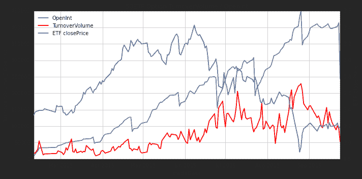
从上图可以看出:
- 期权的交易量基本上是50ETF的反向指标
- 五月之前的疯牛中,期权日交易量处于低位
- 六月中下旬之后的暴跌时间段,期权日交易量高位运行,是不是创个新高
- 8月17日开始的这一周中,大盘风雨飘摇,50ETF探底时,期权交易量创了新高
- 目前来看,期权交易仍然活跃,但是交易量较之前数据有所回落,应该是大盘企稳的节奏
3. 期权的PCR比例
期权分看跌和看涨两种,买入两种不同的期权,代表着对于后市的不同看法,因此可以引进一个量化指标,来表示对后市看衰与看涨的力量的强弱:
- PCR = Put Call Ratio
- PCR可以是关于成交量的PCR,可以是持仓量的PCR,也可以是成交额的PCR
begin = Date(2015, 2, 9)
end = Date.todaysDate()

opt_hist = getOptHistVol(begin, end)
opt_hist.tail(2)
| callVol | putVol | callValue | putValue | callOpenInt | putOpenInt | nearCallVol | nearPutVol | nearCallValue | nearPutValue | ... | nearPutOpenInt | netVol | netValue | netOpenInt | volPCR | valuePCR | openIntPCR | nearVolPCR | nearValuePCR | nearOpenIntPCR | |
|---|---|---|---|---|---|---|---|---|---|---|---|---|---|---|---|---|---|---|---|---|---|
| date | |||||||||||||||||||||
| 2015-09-23 | 50093 | 42910 | 37809117 | 41517121 | 269395 | 144256 | 16603 | 11494 | 6217923 | 10409963 | ... | 50576 | 93003 | 79326238 | 413651 | 0.8566 | 1.0981 | 0.5355 | 0.6923 | 1.6742 | 0.3738 |
| 2015-09-24 | 29352 | 23474 | 21696859 | 22161955 | 146224 | 98350 | 19785 | 19339 | 15693989 | 14549046 | ... | 55217 | 52826 | 43858814 | 244574 | 0.7997 | 1.0214 | 0.6726 | 0.9775 | 0.9270 | 0.8012 |
2 rows × 21 columns
首先,我们来看看成交量PCR和ETF价格走势的关系
## ----------------------------------------------
## 50ETF期权PC比例数据图
fig = plt.figure(figsize=(10,8))
fig.set_tight_layout(True)

# ------ 成交量PC比例 ------
ax = fig.add_subplot(211)
lns1 = ax.plot(opt_hist.index, opt_hist.volPCR, color='r', label = u'volPCR')
ax2 = ax.twinx()
lns2 = ax2.plot(etf.index, etf.closePrice, '-', label = 'closePrice')
lns = lns1+lns2
labs = [l.get_label() for l in lns]
ax.legend(lns, labs, loc=3)
ax.set_ylim(0, 2)

hfmt = dates.DateFormatter('%m')
ax.xaxis.set_major_formatter(hfmt)
ax.grid()
ax.set_xlabel(u"tradeDate(Month)")
ax.set_ylabel(r"PCR")
ax2.set_ylabel(r"ETF ClosePrice")
plt.title('Volume PCR')

# ------ 近月主力期权成交量PC比例 ------
ax = fig.add_subplot(212)
lns1 = ax.plot(opt_hist.index, opt_hist.nearVolPCR, color='r', label = u'nearVolPCR')
ax2 = ax.twinx()
lns2 = ax2.plot(etf.index, etf.closePrice, '-', label = 'closePrice')
lns = lns1+lns2
labs = [l.get_label() for l in lns]
ax.legend(lns, labs, loc=3)
ax.set_ylim(0, 2)

hfmt = dates.DateFormatter('%m')
ax.xaxis.set_major_formatter(hfmt)
ax.grid()
ax.set_xlabel(u"tradeDate(Month)")
ax.set_ylabel(r"PCR")
ax2.set_ylabel(r"ETF ClosePrice")
plt.title('Dominant Contract Volume PCR')

<matplotlib.text.Text at 0x6470990>
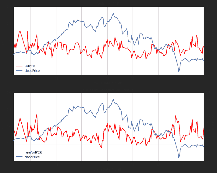
成交量数据图中,上图为全体期权的成交量PCR,下图为近月期权的成交量PCR:
- 上下两图中,PCR的曲线走势基本相似,因为期权交易中,近月期权最为活跃
- ETF价格走势,和PCR走势有比较明显的负相关性
其次,我们来看看持仓量PCR和ETF价格走势的关系
## ----------------------------------------------
## 50ETF期权PC比例数据图
fig = plt.figure(figsize=(10,8))
fig.set_tight_layout(True)

# ------ 持仓量PC比例 ------
ax = fig.add_subplot(211)
lns1 = ax.plot(opt_hist.index, opt_hist.openIntPCR, color='r', label = u'volPCR')
ax2 = ax.twinx()
lns2 = ax2.plot(etf.index, etf.closePrice, '-', label = 'closePrice')
lns = lns1+lns2
labs = [l.get_label() for l in lns]
ax.legend(lns, labs, loc=3)
ax.set_ylim(0, 2)

hfmt = dates.DateFormatter('%m')
ax.xaxis.set_major_formatter(hfmt)
ax.grid()
ax.set_xlabel(u"tradeDate(Month)")
ax.set_ylabel(r"PCR")
ax2.set_ylabel(r"ETF ClosePrice")
plt.title('OpenInt PCR')

# ------ 近月主力期权持仓量PC比例 ------
ax = fig.add_subplot(212)
lns1 = ax.plot(opt_hist.index, opt_hist.nearOpenIntPCR, color='r', label = u'nearVolPCR')
ax2 = ax.twinx()
lns2 = ax2.plot(etf.index, etf.closePrice, '-', label = 'closePrice')
lns = lns1+lns2
labs = [l.get_label() for l in lns]
ax.legend(lns, labs, loc=3)
ax.set_ylim(0, 2)

hfmt = dates.DateFormatter('%m')
ax.xaxis.set_major_formatter(hfmt)
ax.grid()
ax.set_xlabel(u"tradeDate(Month)")
ax.set_ylabel(r"PCR")
ax2.set_ylabel(r"ETF ClosePrice")
plt.title('Dominant Contract OpenInt PCR')

<matplotlib.text.Text at 0x69e5990>
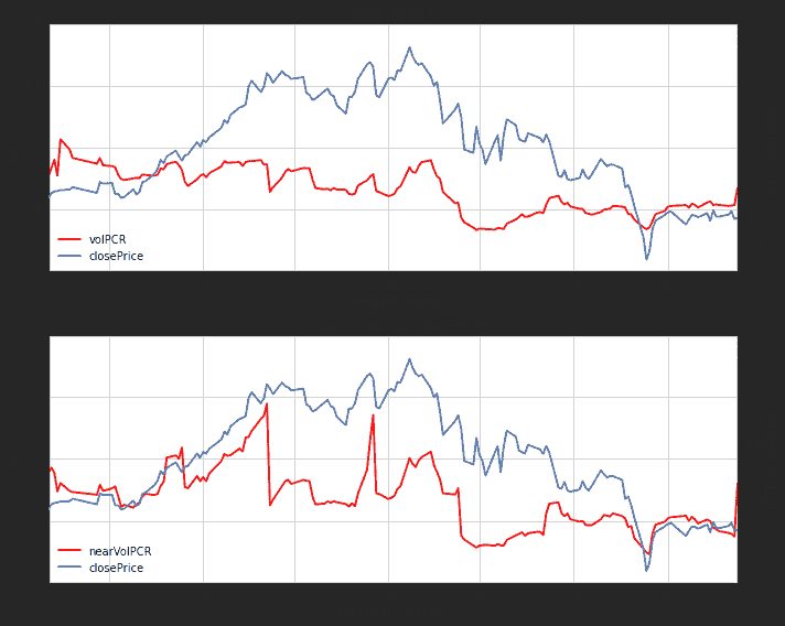
持仓量数据图中,上图为全体期权的持仓量PCR,下图为近月期权的持仓量PCR:
- 上下两图中,PCR的曲线走势基本相似,因为期权交易中,近月期权最为活跃
- 实际上,近月期权十分活跃,使得近月期权的PCR系数变动往往比整体期权PCR变化更剧烈
- ETF价格走势,和PCR走势并无明显的负相关性
- 相反,ETF价格的低点,往往PCR也处于低点,这其实说明:股价大跌之后大家会选择平仓看跌期权
最后,我们来看看成交额PCR和ETF价格走势的关系
## ----------------------------------------------
## 50ETF期权PC比例数据图
fig = plt.figure(figsize=(10,8))
fig.set_tight_layout(True)

# ------ 成交额PC比例 ------
ax = fig.add_subplot(211)
lns1 = ax.plot(opt_hist.index, opt_hist.valuePCR, color='r', label = u'turnoverValuePCR')
ax2 = ax.twinx()
lns2 = ax2.plot(etf.index, etf.closePrice, '-', label = 'closePrice')
lns = lns1+lns2
labs = [l.get_label() for l in lns]
ax.legend(lns, labs, loc=3)
#ax.set_ylim(0, 2)
ax.set_yscale('log')

hfmt = dates.DateFormatter('%m')
ax.xaxis.set_major_formatter(hfmt)
ax.grid()
ax.set_xlabel(u"tradeDate(Month)")
ax.set_ylabel(r"PCR")
ax2.set_ylabel(r"ETF ClosePrice")
plt.title('Turnover Value PCR')

# ------ 近月主力期权成交额PC比例 ------
ax = fig.add_subplot(212)
lns1 = ax.plot(opt_hist.index, opt_hist.nearValuePCR, color='r', label = u'turnoverValuePCR')
ax2 = ax.twinx()
lns2 = ax2.plot(etf.index, etf.closePrice, '-', label = 'closePrice')
lns = lns1+lns2
labs = [l.get_label() for l in lns]
ax.legend(lns, labs, loc=3)
#ax.set_ylim(0, 2)
ax.set_yscale('log')

hfmt = dates.DateFormatter('%m')
ax.xaxis.set_major_formatter(hfmt)
ax.grid()
ax.set_xlabel(u"tradeDate(Month)")
ax.set_ylabel(r"PCR")
ax2.set_ylabel(r"ETF ClosePrice")
plt.title('Dominant Contract Turnover Value PCR')

<matplotlib.text.Text at 0x70ce890>
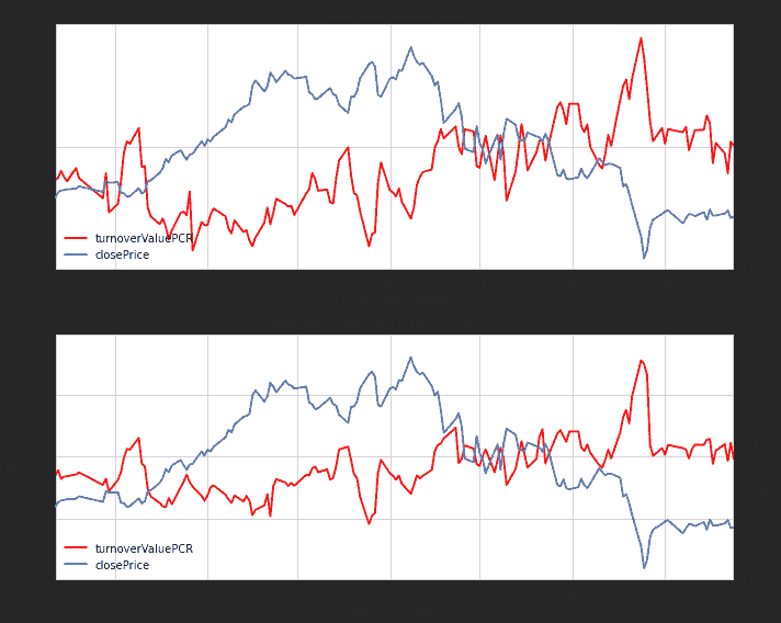
成交额数据图中,上图为全体期权的成交额PCR,下图为近月期权的成交额PCR:
- 上下两图中,PCR的曲线走势基本相似,因为期权交易中,近月期权最为活跃
- 实际上,近月期权PCR指数十分活跃,使得近月期权的PCR系数变动往往比整体期权PCR变化更剧烈
- 相对于成交量和持仓量PCR指标,此处的成交额PCR指标峰值往往很高,上图中近月期权的成交额PCR最大值甚至接近30,这是由于市场恐慌时候,看跌期权成交量本身就大,而交易量大往往将看跌期权的价格大幅抬高
-
ETF价格走势,和PCR走势具有明显的负相关性
-
基于期权成交额PCR的择时策略
根据成交额PCR和ETF价格走势明显的负相关性,我们建立一个非常简单的择时策略:
- PCR下降时,市场情绪趋稳定,全仓买入50ETF
- PCR上升时,恐慌情绪蔓延,清仓观望
start = datetime(2015, 2, 9)                # 回测起始时间
end  = datetime(2015, 9, 21)                # 回测结束时间

hist_pcr = getOptHistVol(start, end)

start = datetime(2015, 2, 9)                # 回测起始时间
end  = datetime(2015, 9, 21)                # 回测结束时间
benchmark = '510050.XSHG'                   # 策略参考标准
universe = ['510050.XSHG']                  # 股票池
capital_base = 100000                       # 起始资金
commission = Commission(0.0,0.0)
refresh_rate = 1

def initialize(account):                    # 初始化虚拟账户状态
    account.fund = universe[0]

def handle_data(account):             # 每个交易日的买入卖出指令
    fund = account.fund
    #  获取回测当日的前一天日期
    dt = Date.fromDateTime(account.current_date)
    cal = Calendar('China.IB')
    cal.addHoliday(Date(2015,9,3))
    cal.addHoliday(Date(2015,9,4))

    last_day = cal.advanceDate(dt,'-1B',BizDayConvention.Preceding)            #计算出倒数第一个交易日
    last_last_day = cal.advanceDate(last_day,'-1B',BizDayConvention.Preceding)  #计算出倒数第二个交易日
    last_day_str = last_day.strftime("%Y-%m-%d")
    last_last_day_str = last_last_day.strftime("%Y-%m-%d")

    # 计算买入卖出信号
    try:
        # 拿取PCR数据
        pcr_last = hist_pcr['valuePCR'].loc[last_day_str]
        pcr_last_last = hist_pcr['valuePCR'].loc[last_last_day_str]
        long_flag = True if (pcr_last - pcr_last_last) < 0 else False
    except:
        long_flag = True

    if long_flag:
        approximationAmount = int(account.cash / account.referencePrice[fund] / 100.0) * 100
        order(fund, approximationAmount)
    else:
        # 卖出时,全仓清空
        order_to(fund, 0)
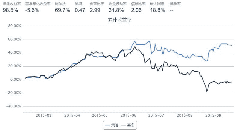
回测结果如上,需要注意的是:
- 期权挂牌时间较短,回测时间短,加上期权市场参与人数少,故而回测结果可能然并卵
- 但是严格根据PCR走势买卖50ETF,还是可以比较好的避开市场大跌的风险
- 不管怎样,PCR可以作为一个择时指标来讨论
- 除了成交额PCR,还可以通过成交量、持仓量、近月成交额等等PCR建立择时策略
